Augmenting Statistical Models with Natural Language Parameters

This is a guest post by my student Ruiqi Zhong, who has some very exciting work defining new families of statistical models that can take natural language explanations as parameters. The motivation is that existing statistical models are bad at explaining structured data. To address this problem, we agument these models with natural language parameters, which can represent interpretable abstract features and be learned automatically.

Imagine the following scenario: It is the year 3024. We are historians trying to understand what happened between 2016 and 2024, by looking at how Twitter topics changed across that time period. We are given a dataset of user-posted images sorted by time, $x_1$, $x_2$ ... $x_T$, and our goal is to find trends in this dataset to help interpret what happened. If we successfully achieve our goal, we would discover, for instance, (1) a recurring spike of images depicting athletes every four years for the Olympics, and (2) a large increase in images containing medical concepts during and after the COVID-19 pandemic.

How do we usually discover temporal trends from a dataset? One common approach is to fit a time series model to predict how the features evolve and then interpret the learned model. However, it is unclear what features to use: pixels and neural image embeddings are high-dimensional and uninterpretable, undermining the goal of extracting explainable trends.

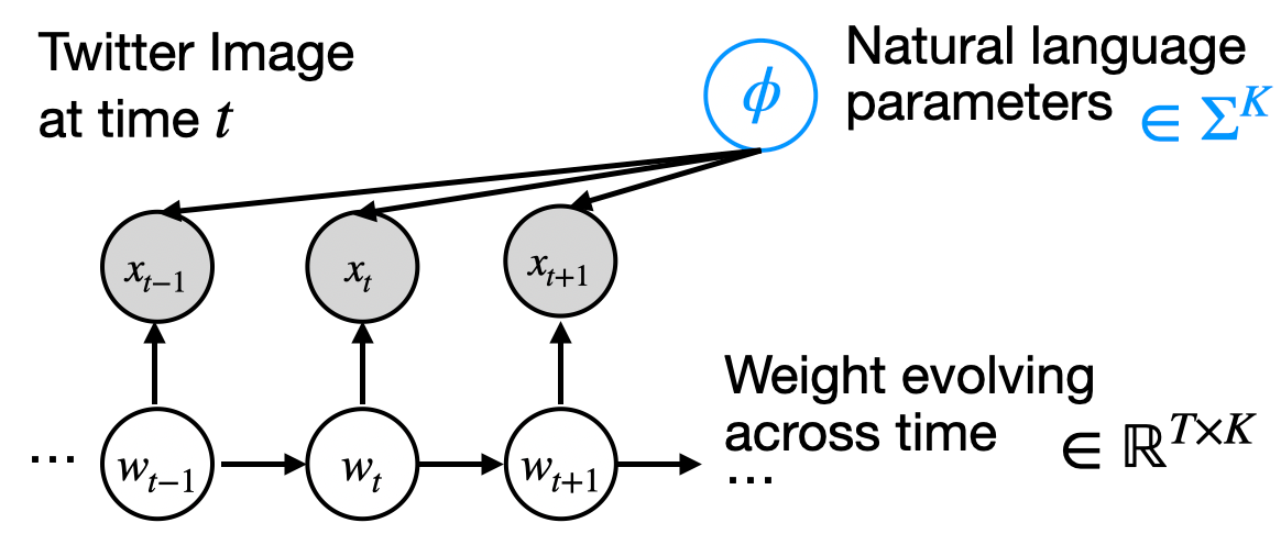
We address this problem by augmenting statistical models with interpretable natural language parameters. The figure below depicts a graphical model representation for the case of time series data. We explain the trends in the observed data [ $x_1$ ... $x_T$] by learning two sets of latent parameters: natural language parameters $\phi$ (the learned features) and real-valued parameters $w$ (the time-varying trends).

• $\phi$: the natural language descriptions of $K$ different topics, e.g. "depicts athletes competing". $\phi$ is an element of $\Sigma$, the universe of all natural language predicates.
• $w_t$: the frequency of each of the K topics at the time $t$.

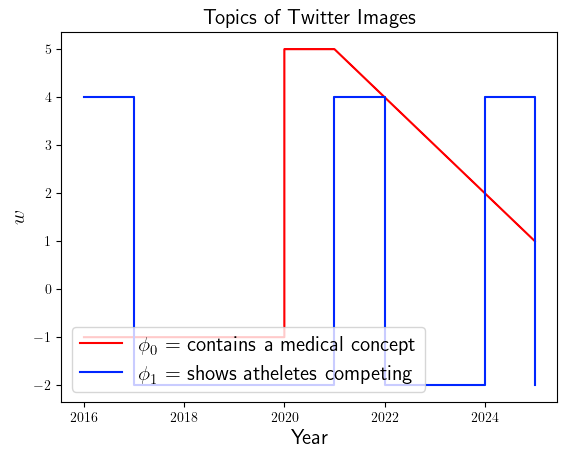
If our model successfully recovers the underlying trends, then we can visualize $w$ and $\phi$ below and see that: 1) more pictures contain medical concepts (red) starting from 2020, and 2) there are recurring (blue) spikes of athletes competing.

In the rest of this post, we will explain in detail how to specify and learn models with natural language parameters and showcase the model on several real-world applications. We will cover:

• A warm-up example of a statistical model with natural language explanations
• A modeling language for specifying natural language parameters
• Applications of our framework, which can be used to specify models for time series, clustering, and applications. We will go over:
  • A machine learning application that uses our time series model to monitor trends in LLM usage
  • A business application that uses our clustering model to taxonomize product reviews
  • A cognitive science application that uses our classification model to explain what images are more memorable for humans

Thanks to Louise Verkin for helping to typeset the post in Ghost format.

Warm-up Example: Logistic Regression with Natural Language Parameters

Instead of understanding topic shifts across the entire time window of 2016-2024, let’s first study a much simpler question: what images are more likely to appear after 2020? The usual way to approach this problem is to,

1. brainstorm some features,
2. extract the real-valued features from each image, and
3. run a logistic regression model on these features to predict the target $Y$ =1 if the image appears after 2020, $Y$ =0 otherwise.

More concretely:

Step 1: Propose different hypotheses about what might make an image more likely to appear after 2020, e.g.:

• a) “depicts a war scene "
• b) “contains a medical concept"
• c) “features Donald Trump"
• d) “is a virus icon "
  ...

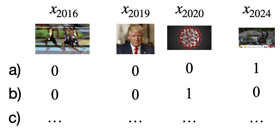
Step 2: For each image $x$, manually check whether it matches each of the hypotheses (a-d), assign a value of 1 if the image matches the description, 0 otherwise. This results in a binary-valued feature vector $f$ for each image $x$. For example:

Consequently, we can obtain a large matrix of binary values:

Step 3: Perform regression analysis: we learn a linear model to predict $y$ (whether the image appears after 2020) based on the real-valued features $f$.

Traditional statistical modeling only focuses on step 3 and learning the weights: these models assume that we already have the hypotheses (a-d) and we have already mapped each image x to a real vector $f$ based on these hypotheses.

However, the first two steps demand significant human effort: the first step requires ad hoc insights to brainstorm these hypotheses, and the second step requires humans to go through a sea of images and laboriously label whether each image matches each hypothesis description. We therefore propose automating the first two steps and learn the natural language descriptions of the hypotheses. ^[1] In other words, we learn not only the real-valued weights $w$ in Figure 3, but also the feature descriptions $\phi$ in the legend.

Formalizing Regression with Natural Language Parameters.

To define any machine learning model, we need to specify the

1. the possible space of parameters for $\phi$ and $w$ and
2. the loss function with respect to the parameters, i.e. $L(\phi, w)$

Parameter Space: The parameters consist of

• $w$: a K-dimensional real-valued weights $W = R^{K}$, which is the same as in standard logistic regression
• $\phi$: A list of K natural language predicates $\Sigma^{K}$.

What is a natural language predicate? It is a natural language string that can extract 0/1 feature values from a sample $x$. The extraction process works as follows: if you give the phi and the image to a human, they will respond with 1 if the image matches phi, and 0 otherwise. ^[2] For example:

Loss Function: Now let’s define the loss function $L(\phi, w)$ for logistic regression:

Given a list of K natural language predicates $\phi$, we can extract a $K$-dimensional binary feature vector. For example:

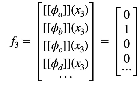
We later use the shorthand $f_3 = [[\phi]](x_3)$. Note that although $[[\phi]](x)$ is expensive to compute since it requires a human in the loop, we can automate this process by prompting a language model with a predicate $\phi_b$ and an image $x_3$, and ask “does the predicate match the image? Yes or no." If the LM responds with yes, then $[[\phi_b]](x_{3})$ = 1, and 0 otherwise.

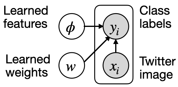
After we have extracted the feature values $f_i$ using $\phi$, we calculate the loss function based on $f_i$ and $w$ in the same way as in standard logistic regression. Here is the graphical model notation for this model:

(A Digression) Fitting the Model. We have written down a well-defined optimization problem to learn a classification model with natural language parameters. But how to minimize the loss and where do these natural language predicates come from?

Due to space limitations, I won’t go into the details, but roughly speaking, we ask an LLM to help us overgenerate candidates of these natural language parameters, and we will later optimize them. For example, we can prompt the language model with several images and directly ask it to propose the candidate natural language parameters:

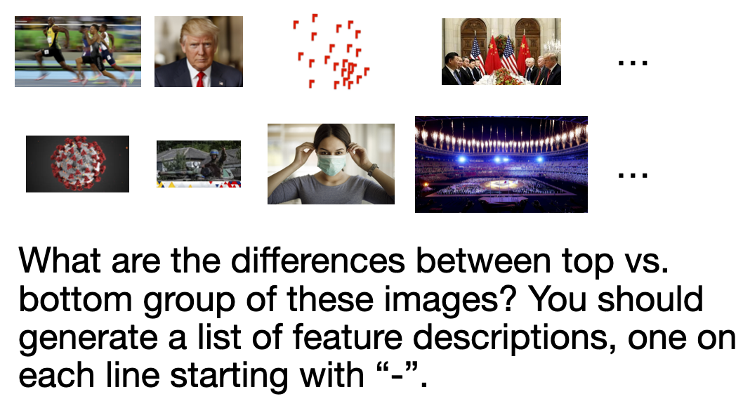
Then the language model would happily spit out a list of feature descriptions as shown above. Many of them are irrelevant, but that’s fine – when we fit the model we can learn not to use those feature descriptions.

A Modeling Language for Specifying More Complex Models

We have formalized a regression model with natural language parameters by defining a loss function based on $w$ and $\phi$. But how do we define the loss function for the time series model, which is much more complicated?

Based on Figure 2, the probability of our model factorizes as follows:

$P(x|w, \phi) = \prod p(w_{t+1}|w_{t}) \prod p(x_t|w_t, \phi)$

The first part is easy to define. Since w_t are real vectors that drift across time, we can define $p(w_{t+1}|w_{t})$ as a normal distribution around $w_{t}$, e.g.

$w_{t+1} = w_{t} + \epsilon_{t}$, where $\epsilon_{t} \in N(0,1)$

To define the second part, we need to define a conditional probability distribution over the images $x$: $p(x|w, \phi)$. We do so by introducing an exponential family:^[3]

Take year 2020 from Figure 3 as an example:
$\phi$ = [“contains a medical concept", “shows athletes competing"]
$w$ = [5, -2]

Therefore, a Twitter image containing a medical concept without atheletes will receive a weight proportional to
$e^{1 * 5 + 0 * (-2)} = e^{5}$

A twitter image showing athletes competing (but not medical) will receive a weight of
$e^{0* 5 + 1 * (-2)} = e^{-2}$

Other images that are neither medical nor atheletic will receive a weight of
$e^{0 * 5 + 0 * (-2)} = e^{0}$

Hence, for the year of 2020, $p(x_{t}|w_{t}, \phi)$ assigns much higher probability to images with a medical concept as $w_0$ significantly increases. Hence, the log likelihood of [$x_1$ ... $x_T$] given w and $\phi$ is the following.

$L(\phi, w) = \sum_{t=1}^{T}-\log (p(x_{t}\mid \phi, w_{t})) + \frac{\lambda}{2} \sum_{t=1}^{T-1}||w_{t} - w_{t+1}||_{2}^{2}$

This concludes the definition of the time series model, which now has a well-defined loss function and parameter space. ^[4] This gives you a flavor of the family of models our framework can define, and now let’s look at real-world applications of our framework.

Example Applications:

We will discuss three applications using our framework, each utilizing a different model with natural language parameters.

• A machine learning application that uses our time series model to monitor trends in LLM usage
• A business application that uses our clustering model to taxonomize product reviews
• A cognitive science application that uses our classification model to explain what images are more memorable to humans

Application 1: monitoring trends in LLM usage via time series modeling

Understanding temporal trends in user queries can assist in forecasting flu outbreaks, preventing self-reinforcing trends in deployed machine learning systems, and identifying new application opportunities. Given user queries to LLMs (e.g. ChatGPT) $x_1$ ... $x_T$, we can use our time series model defined above to identify trends in user queries. We apply the time series model introduced above to discover temporal trends from WildChat, a corpus of real-world user-ChatGPT dialogues. We identify trends below in Figure 11.

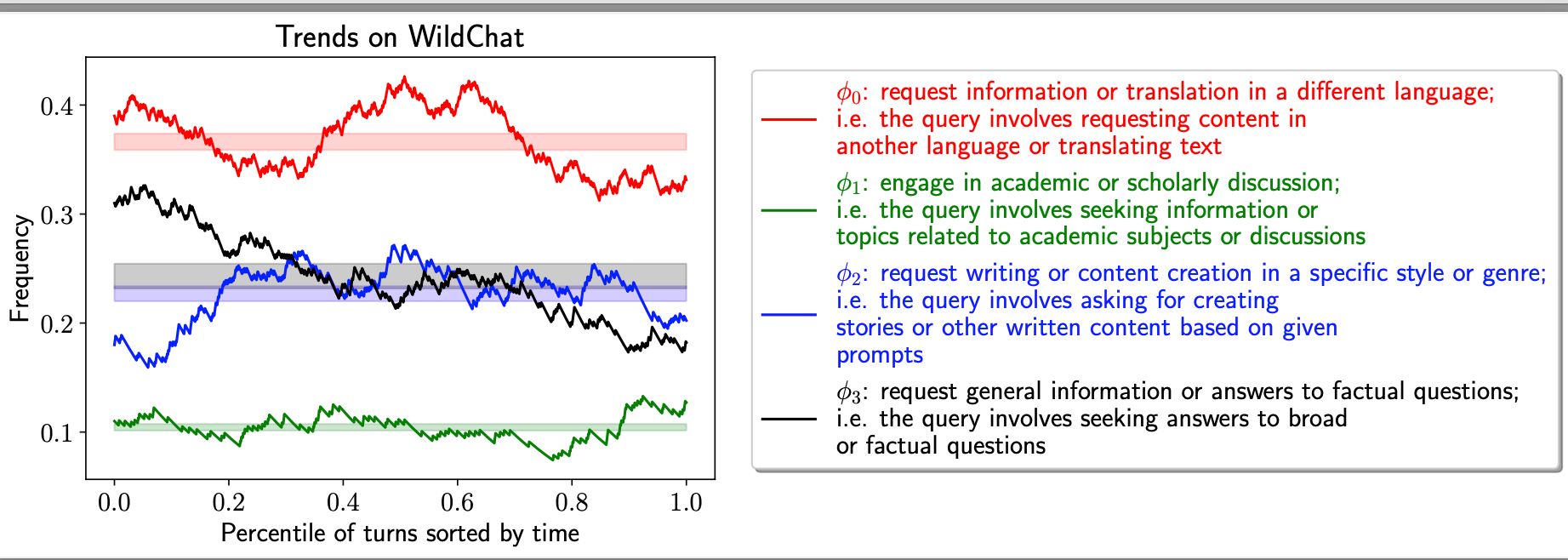
Based on the blue curve, we find that an increasing number of users “requests writing or content creation .... creating stories based on given prompts." This helps motivate the developers to invest more resources to design systems such as Coauthor that assist with this use case.

Application 2: taxonomizing product reviews via clustering

Customer feedback is valuable for businesses to improve their services. However, there might be thousands or even millions of feedback that comment on different aspects of the services, thus making it challenging for business owners to mentally process all of them. It would be ideal to create a taxonomy over these feedback (e.g. Figure 12), but doing so require a lot of human effort to brainstorm the categories based on the customer feedback and carefully match each feedback to a corresponding category.

Fortunately, our framework can automate this tedious process. Our core idea is to define a clustering model where each cluster is associated with a cluster description ($\phi$), and then recursively apply our model to create a tree of clusters and descriptions.

We define our clustering model as follows: we model each observed review as a sample from a cluster; each cluster is parameterized by a description of the cluster, e.g. “complains about produce size or fit", and the cluster is a uniform distribution over all reviews that satisfy this description. Using the graphical model language described above, our clustering model can be represented as Figure 13.

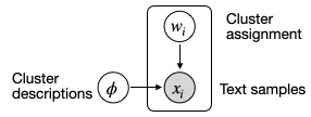
After applying our model recursively among customer reviews, we expect to see a taxonomy similar to the one in Figure 12. Such a method can be broadly applied to other social science/data science applications, such as taxonomizing debate arguments for a political issue or LLM use cases.^[5]

Application 3: Explaining memorable visual features via Classification.

Finally, we look at an interesting cognitive science question: what visual features make an image more memorable for humans? In this application, we are provided with the LaMeM dataset, which contains images $x_1$ ... $x_N$, and each label comes with a label of $y_1$ ... $y_N$ indicating whether it is memorable or not. Our goal is to identify explainable features in image x that increase or decrease the likelihood of $y$ being 1.

We directly plug in the image classification model introduced in our warmup example, and present the findings in Figure 14. Consistent with previous findings, we observe that tranquil scenes make an image less memorable, while emotions and expressions make it more memorable.

Note that this classification model is broadly applicable to many other tasks. For example,

• Explaining a neuron by setting images/text as $x$ and $y=1$ if a neuron is activated by $x$.
• Understanding the differences between two generative models. E.g. an image $x$ has $y=0$ if it comes from StableDiffusionV1 and $y=1$ if it comes from StableDiffusionV2
• Understanding failure modes of a neural network (e.g. ChatGPT). E.g., an input $x$ has $y=0$ if ChatGPT responds to $x$ correctly, and $y=1$ otherwise.

This classification model has a wide range of potential applications, and we refer the reader to Goal Driven Discovery of Distributional Differences via Language Descriptions and Describing Differences in Image Sets with Natural Language for further reading.

Conclusion

Traditional statistical modeling focuses on the “rigid part" of modeling: modeling over real-valued feature values and learning real-valued model weights. However, a significant part of modeling is “soft," and step 1/2 depends on human interpretation. Fortunately, the advance of LLMs make it possible to automate step 1 and 2 as well, thus making it possible to augment statistical models with natural language parameters. In this paper, we introduce a new modeling language to specify these models, thus opening up new application opportunities.