Machine learning is very good at optimizing predictions to match an observed signal --- for instance, given a dataset of input images and labels of the images (e.g. dog, cat, etc.), machine learning is very good at correctly predicting the label of a new image. However, performance can quickly break down as soon as we care about criteria other than predicting observables. There are several cases where we might care about such criteria:
- In scientific investigations, we often care less about predicting a specific observable phenomenon, and more about what that phenomenon implies about an underlying scientific theory.
- In economic analysis, we are most interested in what policies will lead to desirable outcomes. This requires predicting what would counterfactually happen if we were to enact the policy, which we (usually) don't have any data about.
- In machine learning, we may be interested in learning value functions which match human preferences (this is especially important in complex settings where it is hard to specify a satisfactory value function by hand). However, we are unlikely to observe information about the value function directly, and instead must infer it implicitly. For instance, one might infer a value function for autonomous driving by observing the actions of an expert driver.
In all of the above scenarios, the primary object of interest -- the scientific theory, the effects of a policy, and the value function, respectively -- is not part of the observed data. Instead, we can think of it as an unobserved (or "latent") variable in the model we are using to make predictions. While we might hope that a model that makes good predictions will also place correct values on unobserved variables as well, this need not be the case in general, especially if the model is mis-specified.
I am interested in latent variable inference because I think it is a potentially important sub-problem for building AI systems that behave safely and are aligned with human values. The connection is most direct for value learning, where the value function is the latent variable of interest and the fidelity with which it is learned directly impacts the well-behavedness of the system. However, one can imagine other uses as well, such as making sure that the concepts that an AI learns sufficiently match the concepts that the human designer had in mind. It will also turn out that latent variable inference is related to counterfactual reasoning, which has a large number of tie-ins with building safe AI systems that I will elaborate on in forthcoming posts.
The goal of this post is to explain why problems show up if one cares about predicting latent variables rather than observed variables, and to point to a research direction (counterfactual reasoning) that I find promising for addressing these issues. More specifically, in the remainder of this post, I will: (1) give some formal settings where we want to infer unobserved variables and explain why we can run into problems; (2) propose a possible approach to resolving these problems, based on counterfactual reasoning.
1 Identifying Parameters in Regression Problems
Suppose that we have a regression model $p_{\theta}(y \mid x)$, which outputs a probability distribution over $y$ given a value for $x$. Also suppose we are explicitly interested in identifying the "true" value of $\theta$ rather than simply making good predictions about $y$ given $x$. For instance, we might be interested in whether smoking causes cancer, and so we care not just about predicting whether a given person will get cancer ($y$) given information about that person ($x$), but specifically whether the coefficients in $\theta$ that correspond to a history of smoking are large and positive.
In a typical setting, we are given data points $(x_1,y_1), \ldots, (x_n,y_n)$ on which to fit a model. Most methods of training machine learning systems optimize predictive performance, i.e. they will output a parameter $\hat{\theta}$ that (approximately) maximizes $\sum_{i=1}^n \log p_{\theta}(y_i \mid x_i)$. For instance, for a linear regression problem we have $\log p_{\theta}(y_i \mid x_i) = -(y_i - \langle \theta, x_i \rangle)^2$. Various more sophisticated methods might employ some form of regularization to reduce overfitting, but they are still fundamentally trying to maximize some measure of predictive accuracy, at least in the limit of infinite data.
Call a model well-specified if there is some parameter $\theta^*$ for which $p_{\theta^*}(y \mid x)$ matches the true distribution over $y$, and call a model mis-specified if no such $\theta^*$ exists. One can show that for well-specified models, maximizing predictive accuracy works well (modulo a number of technical conditions). In particular, maximizing $\sum_{i=1}^n \log p_{\theta}(y_i \mid x_i)$ will (asymptotically, as $n \to \infty$) lead to recovering the parameter $\theta^*$.
However, if a model is mis-specified, then it is not even clear what it means to correctly infer $\theta$. We could declare the $\theta$ maximizing predictive accuracy to be the "correct" value of $\theta$, but this has issues:
- While $\theta$ might do a good job of predicting $y$ in the settings we've seen, it may not predict $y$ well in very different settings.
- If we care about determining $\theta$ for some scientific purpose, then good predictive accuracy may be an unsuitable metric. For instance, even though margarine consumption might correlate well with (and hence be a good predictor of) divorce rate, that doesn't mean that there is a causal relationship between the two.
The two problems above also suggest a solution: we will say that we have done a good job of inferring a value for $\theta$ if $\theta$ can be used to make good predictions in a wide variety of situations, and not just the situation we happened to train the model on. (For the latter case of predicting causal relationships, the "wide variety of situations" should include the situation in which the relevant causal intervention is applied.)
Note that both of the problems above are different from the typical statistical problem of overfitting. Clasically, overfitting occurs when a model is too complex relative to the amount of data at hand, but even if we have a large amount of data the problems above could occur. This is illustrated in the following graph:
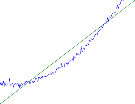
Here the blue line is the data we have ($x,y$), and the green line is the model we fit (with slope and intercept parametrized by $\theta$). We have more than enough data to fit a line to it. However, because the true relationship is quadratic, the best linear fit depends heavily on the distribution of the training data. If we had fit to a different part of the quadratic, we would have gotten a potentially very different result. Indeed, in this situation, there is no linear relationship that can do a good job of extrapolating to new situations, unless the domain of those new situations is restricted to the part of the quadratic that we've already seen.
I will refer to the type of error in the diagram above as mis-specification error. Again, mis-specification error is different from error due to overfitting. Overfitting occurs when there is too little data and noise is driving the estimate of the model; in contrast, mis-specification error can occur even if there is plenty of data, and instead occurs because the best-performing model is different in different scenarios.
2 Structural Equation Models
We will next consider a slightly subtler setting, which in economics is referred to as a structural equation model. In this setting we again have an output $y$ whose distribution depends on an input $x$, but now this relationship is mediated by an unobserved variable $z$. A common example is a discrete choice model, where consumers make a choice among multiple goods ($y$) based on a consumer-specific utility function ($z$) that is influenced by demographic and other information about the consumer ($x$). Natural language processing provides another source of examples: in semantic parsing, we have an input utterance ($x$) and output denotation ($y$), mediated by a latent logical form $z$; in machine translation, we have input and output sentences ($x$ and $y$) mediated by a latent alignment ($z$).
Symbolically, we represent a structural equation model as a parametrized probability distribution $p_{\theta}(y, z \mid x)$, where we are trying to fit the parameters $\theta$. Of course, we can always turn a structural equation model into a regression model by using the identity $p_{\theta}(y \mid x) = \sum_{z} p_{\theta}(y, z \mid x)$, which allows us to ignore $z$ altogether. In economics this is called a reduced form model. We use structural equation models if we are specifically interested in the unobserved variable $z$ (for instance, in the examples above we are interested in the value function for each individual, or in the logical form representing the sentence's meaning).
In the regression setting where we cared about identifying $\theta$, it was obvious that there was no meaningful "true" value of $\theta$ when the model was mis-specified. In this structural equation setting, we now care about the latent variable $z$, which can take on a meaningful true value (e.g. the actual utility function of a given individual) even if the overall model $p_{\theta}(y,z \mid x)$ is mis-specified. It is therefore tempting to think that if we fit parameters $\theta$ and use them to impute $z$, we will have meaningful information about the actual utility functions of individual consumers. However, this is a notational sleight of hand --- just because we call $z$ "the utility function" does not make it so. The variable $z$ need not correspond to the actual utility function of the consumer, nor does the consumer's preferences even need to be representable by a utility function.
We can understand what goes wrong by consider the following procedure, which formalizes the proposal above:
- Find $\theta$ to maximize the predictive accuracy on the observed data, $\sum_{i=1}^n \log p_{\theta}(y_i \mid x_i)$, where $p_{\theta}(y_i \mid x_i) = \sum_z p_{\theta}(y_i, z \mid x_i))$. Call the result $\theta_0$.
- Using this value $\theta_0$, treat $z_i$ as being distributed according to $p_{\theta_0}(z \mid x_i,y_i)$. On a new value $x_+$ for which $y$ is not observed, treat $z_+$ as being distributed according to $p_{\theta_0}(z \mid x_+)$.
As before, if the model is well-specified, one can show that such a procedure asymptotically outputs the correct probability distribution over $z$. However, if the model is mis-specified, things can quickly go wrong. For example, suppose that $y$ represents what choice of drink a consumer buys, and $z$ represents consumer utility (which might be a function of the price, attributes, and quantity of the drink). Now suppose that individuals have preferences which are influenced by unmodeled covariates: for instance, a preference for cold drinks on warm days, while the input $x$ does not have information about the outside temperature when the drink was bought. This could cause any of several effects:
- If there is a covariate that happens to correlate with temperature in the data, then we might conclude that that covariate is predictive of preferring cold drinks.
- We might increase our uncertainty about $z$ to capture the unmodeled variation in $y$.
- We might implicitly increase uncertainty by moving utilities closer together (allowing noise or other factors to more easily change the consumer's decision).
In practice we will likely have some mixture of all of these, and this will lead to systematic biases in our conclusions about the consumers' utility functions.
The same problems as before arise: while we by design place probability mass on values of $z$ that correctly predict the observation $y$, under model mis-specification this could be due to spurious correlations or other perversities of the model. Furthermore, even though predictive performance is high on the observed data (and data similar to the observed data), there is no reason for this to continue to be the case in settings very different from the observed data, which is particularly problematic if one is considering the effects of an intervention. For instance, while inferring preferences between hot and cold drinks might seem like a silly example, the design of timber auctions constitutes a much more important example with a roughly similar flavour, where it is important to correctly understand the utility functions of bidders in order to predict their behaviour under alternative auction designs (the model is also more complex, allowing even more opportunities for mis-specification to cause problems).
3 A Possible Solution: Counterfactual Reasoning
In general, under model mis-specification we have the following problems:
- It is often no longer meaningful to talk about the "true" value of a latent variable $\theta$ (or at the very least, not one within the specified model family).
- Even when there is a latent variable $z$ with a well-defined meaning, the imputed distribution over $z$ need not match reality.
We can make sense of both of these problems by thinking in terms of counterfactual reasoning. Without defining it too formally, counterfactual reasoning is the problem of making good predictions not just in the actual world, but in a wide variety of counterfactual worlds that "could" exist. (I recommend this paper as a good overview for machine learning researchers.)
While typically machine learning models are optimized to predict well on a specific distribution, systems capable of counterfactual reasoning must make good predictions on many distributions (essentially any distribution that can be captured by a reasonable counterfactual). This stronger guarantee allows us to resolve many of the issues discussed above, while still thinking in terms of predictive performance, which historically seems to have been a successful paradigm for machine learning. In particular:
- While we can no longer talk about the "true" value of $\theta$, we can say that a value of $\theta$ is a "good" value if it makes good predictions on not just a single test distribution, but many different counterfactual test distributions. This allows us to have more confidence in the generalizability of any inferences we draw based on $\theta$ (for instance, if $\theta$ is the coefficient vector for a regression problem, any variable with positive sign is likely to robustly correlate with the response variable for a wide variety of settings).
- The imputed distribution over a variable $z$ must also lead to good predictions for a wide variety of distributions. While this does not force $z$ to match reality, it is a much stronger condition and does at least mean that any aspect of $z$ that can be measured in some counterfactual world must correspond to reality. (For instance, any aspect of a utility function that could at least counterfactually result in a specific action would need to match reality.)
- We will successfully predict the effects of an intervention, as long as that intervention leads to one of the counterfactual distributions considered.
(Note that it is less clear how to actually train models to optimize counterfactual performance, since we typically won't observe the counterfactuals! But it does at least define an end goal with good properties.)
Many people have a strong association between the concepts of "counterfactual reasoning" and "causal reasoning". It is important to note that these are distinct ideas; causal reasoning is a type of counterfactual reasoning (where the counterfactuals are often thought of as centered around interventions), but I think of counterfactual reasoning as any type of reasoning that involves making robustly correct statistical inferences across a wide variety of distributions. On the other hand, some people take robust statistical correlation to be the definition of a causal relationship, and thus do consider causal and counterfactual reasoning to be the same thing.
I think that building machine learning systems that can do a good job of counterfactual reasoning is likely to be an important challenge, especially in cases where reliability and safety are important, and necessitates changes in how we evaluate machine learning models. In my mind, while the Turing test has many flaws, one thing it gets very right is the ability to evaluate the accuracy of counterfactual predictions (since dialogue provides the opportunity to set up counterfactual worlds via shared hypotheticals). In contrast, most existing tasks focus on repeatedly making the same type of prediction with respect to a fixed test distribution. This latter type of benchmarking is of course easier and more clear-cut, but fails to probe important aspects of our models. I think it would be very exciting to design good benchmarks that require systems to do counterfactual reasoning, and I would even be happy to incentivize such work monetarily.
Acknowledgements
Thanks to Michael Webb, Sindy Li, and Holden Karnofsky for providing feedback on drafts of this post. If any readers have additional feedback, please feel free to send it my way.