Thanks to Hao Zhang, Kayvon Fatahalian, and Jean-Stanislas Denain for helpful discussions and comments.
Addendum and erratum. See here for an excellent discussion of similar ideas by Kipply Chen. In addition, James Bradbury has pointed out to me that some of the constants in this analysis are wrong, as well as some of the quotes of current hardware capabilities. (See here for some discussion, although we had additional discussion in-person.) I believe that the overall asymptotics below are correct, but the final numbers could plausibly be off by up to an order of magnitude. I hope to eventually fix the numbers, but it's a complicated enough undertaking that it will take some time and care.
Over the last month, I’ve spent a lot of time trying to answer the following question:
How quickly can we perform one forward pass in a transformer model?
By a transformer model, I mean BERT, GPT-3, T5, Chinchilla, or other large language models that use a transformer architecture. By a forward pass, I mean the computation needed to generate the next token given all the tokens so far.[1] By “how quickly”, I mean how much wall clock time elapses between the call to the forward pass and its completion. So, even if I can run 1,000 forward passes in parallel, if each takes 1 second to complete, the answer is 1 second (not 1 millisecond).
One way to attempt answering this is to take the total number of operations in a forward pass and divide by the speed of your favorite GPU in FLOPS (floating-point operations/second). But this is wrong, because you would do better by parallelizing across multiple GPUs.[2]
The question then is really “how effectively can I parallelize a forward pass?” It turns out that this has different answers based on how “wasteful” we’re willing to be, in terms of GPU utilization. If we are willing to utilize only 5% of the GPU (but parallelize across many GPUs), we can perform the forward pass more quickly. So I’ll actually answer two questions:
- How quickly can we perform a forward pass, assuming we require each GPU to have at least 40% utilization relative to roofline FLOPS?[3]
- If we are willing to decrease utilization by a factor of k, how much faster can we perform a forward pass?
To simplify the analysis, I’ll make several assumptions (this is mainly targeted at people who are very familiar with GPU nuts and bolts; don’t worry if you don’t understand them yet):
- [A] Parallelization, both within and across GPUs, is done via matrix tiling, as discussed in the NVIDIA User’s Guide.
- [B] All bottleneck operations can be run at high arithmetic intensity for large batch sizes.
- [C] The constraining resource is always either compute capacity, on-chip memory bandwidth, or network bandwidth of a single machine. In particular, it is not the L2 cache speed, the cross-GPU interconnect, or the ability to route information between far-away nodes in the network.
Assumption A holds for most systems as implemented today, but it’s possible that algorithms such as FlashAttention could lead to better efficiency in the future. Assumption B is actually somewhat false today, because self-attention layers don’t achieve high arithmetic intensity for large context lengths (I’ll discuss this more later). Finally, Assumption C seems likely to hold for well-designed GPU clusters—e.g. under the analysis below, the limiting resource would usually be memory bandwidth for TPU pods, and network bandwidth for a home-grown cluster of A100s.
If Assumption A failed, it would push the time of a forward pass down (because it would mean we’d found a better parallelization strategy). If Assumption C failed, it would push the time up (because there’d be a new resource bottleneck). If Assumption B failed, it would render the question as posed meaningless, because it would not be possible to achieve 40% utilization. However, for whatever utilization was possible to achieve, it would likely push the time down relative to the 40% numbers given below (see here for why).
How Fast for a Forward Pass? The Very Short Answer
The time for a forward pass depends primarily on three properties:
- The number $L$ of layers in the model.
- The speed $C$ of a single GPU, in FLOPS.
- The “ops : bytes” ratio $R$ of the GPU, which is the FLOPS divided by the bandwidth in bytes/second (as measured by either memory reads or network bytes; we’ll assume for now that these are comparable).
Ignoring multiplicative constants, the time for a forward pass is $LR^3/C$. This is because a forward pass primarily consists of $L$ consecutive matrix multiplies, and we can split each matrix multiply into a bunch of $R \times R$ blocks that are each run on a separate GPU, and thus take $R^3$ operations per GPU. $R$ turns out to be the smallest block size at which the GPU can be run at full utilization.
If we are willing to decrease utilization by a factor of $k$, then we can use $\frac{R}{k} \times \frac{R}{k}$ blocks instead. This leads to only needing time $LR^3/Ck^2$. In other words, the time decreases by a factor of $k^2$. Eventually, we would become bottlenecked by latency (which for current clusters is around a few microseconds/layer), but I will ignore that in this analysis.
The Still Short but Technical Answer
I’ll now justify the formulas above, and fill in the multiplicative constants. This section will make sense if you already understand GPUs pretty well, and give you a rough gist if you don’t. In the rest of the document, I’ll explain the relevant facts about GPUs and derive the formulas in a lot more detail.
The full answer depends on four GPU-specific quantities:
- the compute capacity C of the GPU (in FLOPS),
- the memory bandwidth M (in bytes/sec),
- the number N of GPUs per machine, and
- the network bandwidth B, i.e. how quickly information can be sent from one machine to another (also measured in bytes/sec).
In addition, the main thing that matters about the transformer architecture itself is the number $L$ of sequential matrix multiplies that must be performed (this is generally around 2 per layer, so 100-200 for most current architectures).
Interestingly, the answer does not depend on the width of the network. This is because we can always parallelize across more GPUs. The only bottleneck to parallelization is that each GPU needs enough “work” to be utilized efficiently, and this work bottleneck is determined primarily by the GPU’s compute $C$, memory bandwidth $M$, and network bandwidth $B$.
Complete formula. The minimum time to complete one matrix multiply ends up (with some caveats) being
$\text{ElapsedTime} = \left\{ \begin{align*} \frac{54C^2}{M^3} \quad \quad \quad & : \text{ if } B > \frac{2}{3}M\sqrt{N} \\ \frac{8C^2N}{B^2(M-B/\sqrt{N})} & : \text{ else.} \end{align*} \right.$
In this formula, if we are not network bottlenecked then the time grows as $C^2/M^3$, and if we are then it grows as $C^2N/B^2M$.
Finally, if we are willing to decrease utilization by a factor of $k$, we can drive the time down by a factor of $k^2$.
Interpretation for current machines. On current machines, either term in the maximum can dominate: for instance, for an A100 GPU we have C = 312TFLOPS, M = 2TB/s, N=8, and B is variable but perhaps 2TB/S for high-end networks. Then the first term is $0.7 \times 10^{-6}$ and the second is $1.2 \times 10^{-6}$. In other words, on a cluster of A100s, each matrix multiply would take a couple microseconds. This assumes full GPU utilization (in reality it would be 30%-50%) and no latency (in reality around 1.5μs), so in practice it will be higher–perhaps 4-5 microseconds. Since transformers like Chinchilla require 160 consecutive matrix multiplies, the overall time for a forward pass comes out to around 0.7 ms. In contrast, humans take around 250ms to read one word.
Justifying the formula. The rough reason for the formulas above is as follows: ignoring constants, when N=1, we can split any matrix multiplication up into blocks of size $\frac{C}{B} \times \frac{C}{B}$, and process inputs in batches of size $\frac{C}{M}$. For this computation shape, each machine needs to handle $\frac{C^2}{BM}$ incoming network bits per forward pass, $\frac{C^2}{B^2}$ memory reads, and $\frac{C^3}{B^2M}$ floating point operations. Since the first gets handled at a rate of $B$, the second at a rate of $M$, and the third at a rate of $C$, all of them get handled in time $\frac{C^2}{B^2M}$ and hence all resources are fully utilized.
For N>1 GPUs per machine, the input to the entire machine should be blocks of length $\frac{CN}{B}$ with batches of size $\frac{C}{M}$. This gets subdivided further into a $\sqrt{N} \times \sqrt{N}$ grid of blocks of size $\frac{C\sqrt{N}}{B}$, which get sent to each individual GPU. Then we process $\frac{C^2N}{BM}$ network bits (at rate B), $\frac{C^2N}{B^2}$ memory reads per machine (at rate M), and $\frac{C^3N}{B^2M}$ floating point operations per machine (at rate C). In this case each component gets processed in $\frac{C^2N}{B^2M}$ seconds. Finally, the reason we get $\frac{C^2}{M^3}$ in some regimes is that the block size on each GPU also must be at least $\frac{C}{M}$ to avoid being bottlenecked on memory reads.
To sanity check the block tiling scheme above, on an 8xA100 machine the blocks would be 1024x1024 (rounded to the nearest power of 2). Since the dimensionality of many models is around 8192-16384, this means the computation would have to be split across 64-256 machines or 512-2048 total GPUs. This is within the range of possibility, e.g. TPUv4 has 4096 GPUs per node.
Trading off speed and cost. If we scale down both the block and batch size by a factor of $k$, then the utilization drops to $1/k$, but we decrease the work by a factor of $k^3$–therefore, we can complete the multiplication $k^2$ times faster. This works until we start to run into other issues such as memory and network latency, which add up to 1-2 microseconds (and might even increase for large $k$ as it becomes harder to efficiently route information at small block sizes).
Detailed Explanation
A Simple Model of GPU Costs: Transformers as a Stack of Matrix Multiplies
GPUs are used for two important machine learning tasks—training and inference. These have somewhat different requirements:
- At training time, the parameters of the model are constantly being updated, and these updates need to be communicated to the GPUs. Additional state, such as momentum terms for the optimizer, must also be stored and updated. This leads to large memory and large communication costs. In the positive direction, data can be processed simultaneously in large batches. This is important in order to amortize the communication costs, by processing many examples at once per parameter update.
- At inference time, the model parameters are static. They only need to be loaded onto the GPU once at initialization. After that, the main communication cost is processing the input examples (i.e., words) themselves, which is much cheaper because it involves vectors (activations) rather than matrices (weights). To improve parallelization, the model weights are sharded across multiple GPUs, with each GPU storing and processing a contiguous block of a weight matrix (as described in more detail below). In addition to parallelization, sharding is important because the full set of model weights is often too big to fit onto a single GPU.
I’ll next dive into inference in more detail, since inference time is what governs the serial time per word.
As an abstraction, we’ll think of a neural network as performing many consecutive matrix-vector multiplies, interleaved with a number of cheaper non-linear operations. The matrix-vector multiplies are the dominant cost, so we’ll focus on those and ignore the others. As a concrete example, consider a transformer model, which primarily consists of self-attention and feed-forward blocks. A self-attention block looks like this:
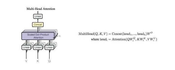
The main cost is the 3 linear blocks for the values (V), keys (K), and queries (Q). Each involves multiplying a d-dimensional vector by a dxd matrix (total cost $\approx 3d^2$). For context length C, the attention block involves computing C d-dimensional vector-vector inner products (total cost $\approx Cd$) together with a normalization and softmax operation (total cost O(C)), and finally taking a sum of d-dimensional vectors weighted by the C attention weights (total cost $\approx Cd$).[4] A typical value of d is 8192-16384, while a typical value of C is 2048. So the matrix multiplies are 6-12 times more expensive than the next most expensive term.[5]
Note that the cost of the matrix-vector multiplies is directly proportional to the size of the matrices. This means that the total cost in FLOPs of a forward-pass is essentially proportional to the number of parameters in the model, and works out to 2 floating-point operations per parameter (1 multiply + 1 add). This will generally be the case in the absence of recurrence or other forms of weight sharing, though I expect weight sharing to eventually be present in future models.
Cost of Implementing Matrix-Vector Multiplies on GPUs
Implementing a matrix-vector multiply on a GPU has four major costs:
- We need to communicate and store the parameters of the matrix (once, at initialization).
- For each new input, we need to communicate the input vector to the GPU (and send the output vector back to RAM or to other GPUs). This cost can be ignored if the matrix for the previous/next multiply is on the same GPU.
- We need to read the data from on-chip memory.
- We need to perform the actual multiply operation.
I’ll ignore (1.), since it can be amortized away, and focus on how costs (2.-4.) add up in practice. I’ll start by imagining that all operations happen on a single GPU, then consider parallelizing across multiple GPUs.
Warm-up: Single GPU, No Batching
As a simple example, let’s consider a 4096-dimensional vector, which needs to get multiplied by a sequence of $L$ $4096 \times 4096$ matrices, with $L=16$. Each matrix entry is 2 bytes[6], so we’re using $2^{12+12+4+1} = 2^{29}$ bytes in total, or 0.5GB. Most GPUs have at least 10GB of memory, so this fits easily onto a single chip.
For each new input to the model, we need to communicate one 4096-dimensional vector to the GPU. So that’s 8192 bytes of communication. In addition, we need 2 x 16 x (4096 x 4096) FLOPs to actually perform the 16 matrix-vector products (2 FLOPs per matrix entry), or 0.5GFLOPs. We similarly need to perform 0.5GB of memory reads to load the matrix into memory (plus a much smaller number of reads and writes for the vector input and output). Thus, overall we need:
- ~8KB of communication
- ~0.5GB of memory accesses
- ~0.5GFLOPs of computation
How long does each part take? Let’s consider an A100 GPU, which has 312TFLOP/s of computation, 1.5TB/s of memory bandwidth, and (depending on network setup) ~400GB/s of network bandwidth. Then communication takes 8KB/(400GB/s) = 0.02μs. Memory takes 0.5GB/(1.5TB/s) = 330μs. And computation takes 0.5GFLOP/(312TF/s) = 1.6μs.
From a cost perspective, this is terrible! The system is totally bottlenecked on memory reads—computation takes only 0.5% of the time that it takes to read from memory, which means that the GPU is only running at 0.5% utilization. In terms of cost, this means you are overpaying for your GPU by a factor of 200.
To solve this, we process inputs in batches. Suppose that instead of reading one input, we read 256 inputs at once[7], represented as a 4096 x 256 vector. Then our costs change as follows:
- Communication: 2MB (was 8KB)
- Memory: 0.56GB (was 0.5GB—the extra .06 is from reading and writing the 4096 x 256 input and output at each layer)
- Compute: 128GFLOPs (was 0.5GFLOPs)
Now how long does each part take? Communication is now 5μs, memory is 350μs, and computation is 400μs. Now memory and computation take about the same time, and the GPU can run at 100% utilization (in theory). In addition, the serial time barely increased. It is now 400μs (or 25μs/layer), up from 330μs before.
Tiling Across GPUs
If we want to run the computation as fast as possible, we probably want to parallelize our computation across more than one GPU. For now I’m just going to focus on a single 4096 x 4096 matrix multiplication (i.e. one layer of the model).
Let’s suppose that instead of one A100 GPU, I have four A100 GPUs. I can think of these GPUs as a 2x2 grid and “tile” my multiplication across them: processing a 2048 x 2048 block of the matrix in each tile of the grid.
To implement this, given my input (still a 4096 x 256 vector), I do the following:
- Split the input into two 2048 x 256 vectors, $u_1$ and $u_2$.
- Send $u_1$ to the first two machines (getting outputs $v_{11}$ and $v_{12}$) and $u_2$ to the second two machines (getting outputs $v_{21}$ and $v_{22}$).
- As a post-processing step, add together $v_1 = v_{11}+v_{12}$ and $v_2 = v_{21}+v_{22}$, then concatenate $v_1$ and $v_2$ into a single output vector $v$.
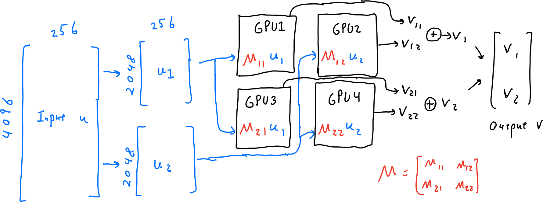
Pretty much all the work here happens in step (2.). In this step, each machine must receive and send a 2048 x 256 vector (~2MB total), read or write matrices of size 2048x256, 2048x2048, and 2048x256 (~10MB), and run 2048x2048x256 add-multiply operations (~2GFLOPs). For the same hardware specs as before, this comes out to 5μs for communication, 6μs for memory, and 6μs for computation. Relative to the 25μs/layer from before, we’ve achieved a 4x speed-up due to parallelizing across 4 GPUs.
In general, we can continue to parallelize across more and more GPUs by splitting into smaller and smaller blocks, as long as we don’t end up bottlenecked by memory or communication costs. In the next section, we’ll carefully count the communication, memory, and compute usage as a function of the block and batch size, and analyze what range they need to be in to achieve full GPU utilization.
Detailed Count of Operation Costs
In general, let’s suppose that we have a large $d \times d$ matrix multiply, and we want to split it up into smaller blocks. Let $m$ denote the block size, and suppose that we process inputs in batches of size $b$. Then we need $(d/m)^2$ GPUs in total, and each individual GPU performs the following operations:
- Receives an incoming matrix of length m x b (a batch of b vectors of length m).
- Multiplies this m x b matrix by a fixed m x m matrix that is stored on the GPU (i.e., a single block of the weight matrix of the model).
- Outputs a vector of length m x b.
As in the previous section, there is also some pre- and post-processing to split and combine the d x 1 vectors into m x 1 vectors, but we will ignore those as they generally only contribute lower-order terms.
Overall, this requires $4mb$ bytes of network communication ($mb$ 16-bit floats on both input and output, and each float is two bytes). It requires $4mb + 2m^2$ memory accesses (each number is again 2 bytes, and we need to read an $m \times b$ and $m \times m$ matrix and write an $m \times b$ matrix). Finally, it requires $2m^2b$ floating point operations. Therefore, the total elapsed time is
$\quad \quad \quad \max\Big(\frac{4mb}{B}, \frac{4mb+2m^2}{M}, \frac{2m^2b}{C}\Big) \quad \quad \quad (\star)$
To avoid being memory constrained and reach full GPU utilization, the third term must be at least the second term (see NVIDIA docs for discussion). Therefore, we have the constraint
$\frac{4mb+2m^2}{2m^2b} \leq \frac{M}{C}$
By the same token, to avoid being communication constrained we should have
$\frac{4mb}{2m^2b} \leq \frac{B}{C}$
This second equation is easy to solve and implies the block size $m$ should be at least $\frac{2C}{B}$ to avoid communication bottlenecks.
The first equation is a bit trickier. It works out to $\frac{2}{m} + \frac{1}{b} \leq \frac{M}{C}$. Since we already know $m$, this comes out to $\frac{1}{b} \leq \frac{M-B}{C}$, so the block size $b$ should be at least $\frac{C}{M-B}$. Plugging back into the formula $(\star)$, the total elapsed time is
$\frac{2m^2b}{C} = \frac{8C^2}{B^2(M-B)}$
But wait! This equation becomes infinite if $M=B$. What went wrong? Well, we set $m$ equal to $\frac{2C}{B}$, but actually it just needs to be at least this large. In fact, it turns out that we always want $m$ to be at least as large as the batch size $b$. So aside from setting $m=\frac{2C}{B}$, the alternative is to set $m$ equal to $b$, in which case we get $m=b=\frac{3C}{M}$. This yields an elapsed time of $\frac{54C^2}{M^3}$. We end up with this elapsed time whenever $M \leq 1.5B$.
One Machine, Multiple GPUs
In many cases, we have more than one GPU on a machine. Then communication splits into two costs: communication between RAM and the GPU (or between GPUs), and communication between this machine and other machines. Typically, within-machine communication is fast compared to between-machine communication, so we’ll treat cross-GPU (within-machine) communication as “free”, while cross-machine communication has a network bandwidth of B.
Suppose that each machine has N GPUs. Then in the simplest accounting, each individual GPU only gets $\frac{B}{N}$ of the network bandwidth, and it’s as if we’re in the single-GPU case above, but with bandwidth $\frac{B}{N}$ instead of $B$.
However, it turns out we can do better. If instead of processing $N$ arbitrary $m \times m$ blocks of the $d \times d$ matrix, we process a $\sqrt{N} \times \sqrt{N}$ grid of $m \times m$ blocks, then we can treat the entire computation as a $m\sqrt{N} \times m\sqrt{N}$ block. In particular, we only need to process input and output vectors of length $m\sqrt{N}$, rather than $mN$. This means that each machine effectively gets network bandwidth $B/\sqrt{N}$, rather than $B/N$ (here I’m assuming $N$ is a perfect square).
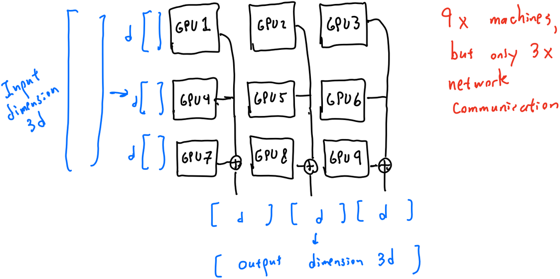
This leads to the final formula, which is equivalent to the single-machine formula but replaces $B$ with $B/\sqrt{N}$. We repeat it here for completeness:
$\text{ElapsedTime} = \left\{ \begin{align*} \frac{54C^2}{M^3} \quad \quad \quad & : \text{ if } B > \frac{2}{3}M\sqrt{N} \\ \frac{8C^2N}{B^2(M-B/\sqrt{N})} & : \text{ else.} \end{align*} \right.$
Remember that this is the elapsed time for a single matrix multiply. To get the elapsed time for a forward pass, we need to multiply by $L$, which for transformers is usually twice the number of layers.
More on Memory Constraints
This entire discussion so far assumes that we can actually reach 100% utilization by increasing the batch size. However, some operations are not effectively batchable and end up constrained on memory reads for large batch sizes. For transformers, this happens when computing the self-attention weights, which is a lower-order term for small batch size but becomes the bottleneck for large batch size and context length.
There are a few ways to think about this. First, we could argue that such bottlenecks probably go away (or at least don't accumulate) in the long run. For instance, Google's PaLM model modifies the self-attention block to partially mitigate this issue. I don't think this argument entirely holds, since most optimizations target training costs rather than inference costs, but I do think there's some truth to it.
Alternatively, we could take such bottlenecks as given. Perhaps we actually can't hope for more than (say) 10% GPU utilization, which also means that the theoretical batch size of $\frac{3C}{M}$ is much larger than necessary (since we're only trying to hit 10% rather than 100% utilization). This is effectively the same as setting $k = 10$---achieving only 10% utilization but running the computation 100 times faster. In other words, if there are unavoidable memory bottlenecks, our analysis still generally holds, except that we are forced to set $k$ to some value larger than $1$.
Overall, then, I don't think that memory constraints (from self-attention or other hypothetical blocks) significantly alter the analysis. We can either assume they go away over time, or just restrict our analysis to a certain regime of the GPU utilization $\frac{1}{k}$.
Other Possible Bottlenecks
In reality, cross-machine communication and GPU memory bandwidth are not the only possible bottlenecks. For instance, we could be bottlenecked by cross-GPU communication within a machine (discussed above), or by L1 or L2 cache speed. But in practice, these are rarely the bottlenecks, so I’ve focused above on the two cases that typically matter. The main other case that I think could matter is end-to-end network communication---it could be that each machine has enough network bandwidth, but the overall cluster has a network topology that makes it hard to efficiently route packets. This seems possible to me, but I also think that well-designed clusters can probably avoid this, so for simplicity I ignored it in my analysis.
In addition, I’ve made a number of idealized assumptions, such as that C/B and C/M are integers, that all quantities nicely divide each other, and implicitly that many quantities are powers of 2 or divisible by powers of 2 (needed to get good cache performance; not discussed here). I’ve also ignored a number of smaller operations like the nonlinearities in each layer, and mostly ignored network and memory latency. I’m basically folding these all into the “30%-50% GPU utilization” fudge factor, which should usually be attainable in practice, but often requires good systems engineering. So, this post isn’t a recipe for actually parallelizing your forward pass, but it should give a good idea of how quickly it can be done in principal.
Summary
Forward passes can be parallelized to a fairly large degree before running into memory or network bottlenecks. Roughly speaking, the time for a single matrix multiply grows quadratically with the GPU FLOPS, and decreases cubically with the network/memory bandwidth. We gave an exact formula (under idealized assumptions) that counts the actual floating-point operations, memory reads/writes, and network usage, and determines the regimes when memory vs. network become the bottleneck resource.
In the next post, I'll apply this formula to forecast how fast not just today's models, but also future ones, can be run.
Specifically, I assume the model also generated all the previous tokens and that their activation vectors are cached, so it only needs to compute activation vectors for the current position. ↩︎
In fact, you are also forced to use multiple GPUs, because state-of-the-art models don’t fit into a single GPU’s memory. ↩︎
I chose 40% to be a “decent” level–generally attainable after working hard to optimize out bottlenecks, but below the best possible. ↩︎
Technically speaking, for a context window of size C, all costs should be multiplied by C (since we need to do all these computations for each token in the context). However, assuming that we are reading or writing a sequence of consecutive words, the previous C-1 tokens have already been computed and their results can be cached and re-used. Naive caching increases memory costs by a nontrivial amount, but there are tricks such as rematerialization that reduce this at a ~33% overhead in computation. ↩︎
One very important caveat is that the self-attention operations cannot be efficiently batched, because the key and query vectors both change for each batch item. This means that self-attention becomes memory-bottlenecked faster than other operations, as I’ll discuss in more detail later. ↩︎
Assuming bfloat16 format, which is typically used to speed up inference. ↩︎
I chose 256 because it was the power of 2 closest to 200, which was the amount by which we were underutilizing the GPU. ↩︎