I just finished presenting my recent paper on stochastic verification at RSS 2011. There is a conference version online, with a journal article to come later. In this post I want to go over the problem statement and my solution.
Problem Statement
Abstractly, the goal is to be given some sort of description of a system, and of a goal for that system, and then verify that the system will reach that goal. The difference between our work and a lot (but not all) of the previous work is that we want to work with an explicit noise model for the system. So, for instance, I tell you that the system satisfies
$dx(t) = f(x) dt + g(x) dw(t),$
where $f(x)$ represents the nominal dynamics of the system, $g(x)$ represents how noise enters the system, and $dw(t)$ is a standard Wiener process (the continuous-time version of Gaussian noise). I would like to, for instance, verify that $h(x(T)) < 0$ for some function $h$ and some final time $T$. For example, if $x$ is one-dimensional then I could ask that $x(10)^2-1 < 0$, which is asking for $x$ to be within a distance of $1$ of the origin at time $10$. For now, I will focus on time-invariant systems and stability conditions. This means that $f$ and $g$ are not functions of $t$, and the condition we want to verify is that $h(x(t)) < 0$ for all $t \in [0,T]$. However, it is not too difficult to extend these ideas to the time-varying case, as I will show in the results at the end.
The tool we will use for our task is a supermartingale, which allows us to prove bounds on the probability that a system leaves a certain region.
Supermartingales
Let us suppose that I have a non-negative function $V$ of my state $x$ such that $\mathbb{E}[\dot{V}(x(t))] \leq c$ for all $x$ and $t$. Here we define $\mathbb{E}[\dot{V}(x(t))]$ as
$\lim\limits_{\Delta t \to 0^+} \frac{\mathbb{E}[V(x(t+\Delta t)) \mid x(t)]-V(x(t))}{\Delta t}.$
Then, just by integrating, we can see that $\mathbb{E}[V(x(t)) \mid x(0)] \leq V(x(0))+ct$. By Markov's inequality, the probability that $V(x(t)) \geq \rho$ is at most $\frac{V(x(0))+ct}{\rho}$.
We can actually prove something stronger as follows: note that if we re-define our Markov process to stop evolving as soon as $V(x(t)) = \rho$, then this only sets $\mathbb{E}[\dot{V}]$ to zero in certain places. Thus the probability that $V(x(t)) \geq \rho$ for this new process is at most $\frac{V(x(0))+\max(c,0)t}{\rho}$. Since the process stops as soon as $V(x) \geq \rho$, we obtain the stronger result that the probability that $V(x(s)) \geq \rho$ for any $s \in [0,t]$ is at most $\frac{V(x(0))+\max(c,0)t}{\rho}$. Finally, we only need the condition $\mathbb{E}[\dot{V}] \leq c$ to hold when $V(x) < \rho$. We thus obtain the following:
Theorem. Let $V(x)$ be a non-negative function such that $\mathbb{E}[\dot{V}(x(t))] \leq c$ whenever $V(x) < \rho$. Then with probability at least $1-\frac{V(x(0))+\max(c,0)T}{\rho}$, $V(x(t)) < \rho$ for all $t \in [0,T)$.
We call the condition $\mathbb{E}[\dot{V}] \leq c$ the supermartingale condition, and a function that satisfies the martingale condition is called a supermartingale. If we can construct supermartingales for our system, then we can bound the probability that trajectories of the system leave a given region.
NOTE: for most people, a supermartingale is something that satisfies the condition $\mathbb{E}[\dot{V}] \leq 0$. However, this condition is often impossible to satisfy for systems we might care about. For instance, just consider exponential decay driven by Gaussian noise:
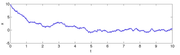
Once the system gets close enough to the origin, the exponential decay ceases to matter much and the system is basically just getting bounced around by the Gaussian noise. In particular, if the system is ever at the origin, it will get perturbed away again, so you cannot hope to find a non-constant function of $x$ that is decreasing in expectation everywhere (just consider the global minimum of such a function: in all cases, there is a non-zero probability that the Gaussian noise will cause $V(x)$ to increase, but a zero probability that $V(x)$ will decrease because we are already at the global minimum this argument doesn't actually work, but I am pretty sure that my claim is true at least subject to sufficient technical conditions).
Applying the Martingale Theorem
Now that we have this theorem, we need some way to actually use it. First, let us try to get a more explicit version of the Martingale condition for the systems we are considering, which you will recall are of the form $dx(t) = f(x) dt + g(x) dw(t)$. Note that $V(x+\Delta x) = V(x) + \frac{\partial V}{\partial x} \Delta x + \frac{1}{2}Trace\left(\Delta x^T \frac{\partial^2 V}{\partial x^2}\Delta x\right)+O(\Delta x^3)$.
Then $\mathbb{E}[\dot{V}(x)] = \lim_{\Delta t \to 0^+} \frac{\frac{\partial V}{\partial x} \mathbb{E}[\Delta x]+\frac{1}{2}Trace\left(\mathbb{E}[\Delta x^T \frac{\partial^2 V}{\partial x^2}\Delta x\right)+O(\Delta x^3)}{\Delta t}$. A Wiener process satisfies $\mathbb{E}[dw(t)] = 0$ and $\mathbb{E}[dw(t)^2] = dt$, so only the nominal dynamics ($f(x)$) affect the limit of the first-order term while only the noise ($g(x)$) affects the limit of the second-order term (the third-order and higher terms in $\Delta x$ all go to zero). We thus end up with the formula
$\mathbb{E}[\dot{V}(x)] = \frac{\partial V}{\partial x}f(x)+\frac{1}{2}Trace\left(g(x)^T\frac{\partial^2 V}{\partial x^2}g(x)\right).$
It is not that difficult to construct a supermartingale, but most supermartingales that you construct will yield a pretty poor bound. To illustrate this, consider the system $dx(t) = -x dt + dw(t)$. This is the example in the image from the previous section. Now consider a quadratic function $V(x) = x^2$. The preceding formula tells us that $\mathbb{E}[\dot{V}(x)] = -2x^2+1$. We thus have $\mathbb{E}[\dot{V}(x)] \leq 1$, which means that the probability of leaving the region $x^2 < \rho$ is at most $\frac{x(0)^2+T}{\rho}$. This is not particularly impressive: it says that we should expect $x$ to grow roughly as $\sqrt{T}$, which is how quickly $x$ would grow if it was a random walk with no stabilizing component at all.
One way to deal with this is to have a state-dependent bound $\mathbb{E}[\dot{V}] \leq c-kV$. This has been considered for instance by Pham, Tabareau, and Slotine (see Lemma 2 and Theorem 2), but I am not sure whether their results still work if the supermartingale condition only holds locally instead of globally; I haven't spent much time on this, so they could generalize quite trivially.
Another way to deal with this is to pick a more quickly-growing candidate supermartingale. For instance, we could pick $V(x) = x^4$. Then $\mathbb{E}[\dot{V}] = -4x^4+6x^2$, which has a global maximum of $\frac{9}{4}$ at $x = \frac{\sqrt{3}}{2}$. This bounds then says that $x$ grows at a rate of at most $T^{\frac{1}{4}}$, which is better than before, but still much worse than reality.
We could keep improving on this bound by considering successively faster-growing polynomials. However, automating such a process becomes expensive once the degree of the polynomial gets large. Instead, let's consider a function like $V(x) = e^{0.5x^2}$. Then $\mathbb{E}[\dot{V}] = e^{0.5x^2}(0.5-0.5x^2)$, which has a maximum of 0.5 at x=0. Now our bound says that we should expect x to grow like $\sqrt{\log(T)}$, which is a much better growth rate (and roughly the true growth rate, at least in terms of the largest value of $\|x\|$ over the time interval $[0,T]$).
This leads us to our overall strategy for finding good supermartingales. We will search across functions of the form $V(x) = e^{x^TSx}$ where $S \succeq 0$ is a matrix (the $\succeq$ means "positive semidefinite", which roughly means that the graph of the function $x^TSx$ looks like a bowl rather than a saddle/hyperbola). This begs two questions: how to upper-bound the global maximum of $\mathbb{E}[\dot{V}]$ for this family, and how to search efficiently over this family. The former is done by doing some careful work with inequalities, while the latter is done with semidefinite programming. I will explain both below.
Upper-bounding $\mathbb{E}[\dot{V}]$
In general, if $V(x) = e^{x^TSx}$, then $\mathbb{E}[\dot{V}(x)] = e^{x^TSx}\left(2x^TSf(x)+Trace(g(x)^TSg(x))+2x^TSg(x)g(x)^TSx\right)$. We would like to show that such a function is upper-bounded by a constant $c$. To do this, move the exponential term to the right-hand-side to get the equivalent condition $2x^TSf(x)+Trace(g(x)^TSg(x))+2x^TSg(x)g(x)^TSx \leq ce^{-x^TSx}$. Then we can lower-bound $e^{-x^TSx}$ by $1-x^TSx$ and obtain the sufficient condition
$c(1-x^TSx)-2x^TSf(x)-Trace(g(x)^TSg(x))-2x^TSg(x)g(x)^TSx \geq 0.$
It is still not immediately clear how to check such a condition, but somehow the fact that this new condition only involves polynomials (assuming that f and g are polynomials) seems like it should make computations more tractable. This is indeed the case. While checking if a polynomial is positive is NP-hard, checking whether it is a sum of squares of other polynomials can be done in polynomial time. While sum of squares is not the same as positive, it is a sufficient condition (since the square of a real number is always positive).
The way we check whether a polynomial p(x) is a sum of squares is to formulate it as the semidefinite program: $p(x) = z^TMz, M \succeq 0$, where $z$ is a vector of monomials. The condition $p(x) = z^TMz$ is a set of affine constraints on the entries of $M$, so that the above program is indeed semidefinite and can be solved efficiently.
Efficiently searching across all matrices S
We can extend on the sum-of-squares idea in the previous section to search over $S$. Note that if $p$ is a parameterized polynomial whose coefficient are affine in a set of decision variables, then the condition $p(x) = z^TMz$ is again a set of affine constraints on $M$. This almost solves our problem for us, but not quite. The issue is the form of $p(x)$ in our case:
$c(1-x^TSx)-2x^TSf(x)-Trace(g(x)^TSg(x))-2x^TSg(x)g(x)^TSx$
Do you see the problem? There are two places where the constraints do not appear linearly in the decision variables: $c$ and $S$ multiply each other in the first term, and $S$ appears quadratically in the last term. While the first non-linearity is not so bad ($c$ is a scalar so it is relatively cheap to search over $c$ exhaustively), the second non-linearity is more serious. Fortunately, we can resolve the issue with Schur complements. The idea behind Schur complements is that, assuming $A \succeq 0$, the condition $B^TA^{-1}B \preceq C$ is equivalent to $\left[ \begin{array}{cc} A & B \ B^T & C \end{array} \right] \succeq 0$. In our case, this means that our condition is equivalent to the condition that
$\left[ \begin{array}{cc} 0.5I & g^TSx \ x^TSg & c(1-x^TSx)-2x^TSf(x)-Trace(g(x)^TSg(x))\end{array} \right] \succeq 0$
where $I$ is the identity matrix. Now we have a condition that is linear in the decision variable $S$, but it is no longer a polynomial condition, it is a condition that a matrix polynomial be positive semidefinite. Fortunately, we can reduce this to a purely polynomial condition by creating a set of dummy variables $y$ and asking that
$y^T\left[ \begin{array}{cc} 0.5I & g^TSx \ x^TSg & c(1-x^TSx)-2x^TSf(x)-Trace(g(x)^TSg(x))\end{array} \right]y \geq 0$
We can then do a line search over $c$ and solve a semidefinite program to determine a feasible value of $S$. If we care about remaining within a specific region, we can maximize $\rho$ such that $x^TSx < \rho$ implies that we stay in the region. Since our bound on the probability of leaving the grows roughly as $ce^{-\rho}T$, this is a pretty reasonable thing to maximize (we would actually want to maximize $\rho-\log(c)$, but this is a bit more difficult to do).
Oftentimes, for instance if we are verifying stability around a trajectory, we would like $c$ to be time-varying. In this case an exhaustive search is no longer feasible. Instead we alternate between searching over $S$ and searching over $c$. In the step where we search over $S$, we maximize $\rho$. In the step where we search over $c$, we maximize the amount by which we could change $c$ and still satisfy the constraints (the easiest way to do this is by first maximizing $c$, then minimizing $c$, then taking the average; the fact that semidefinite constraints are convex implies that this optimizes the margin on $c$ for a fixed $S$).
A final note is that systems are often only stable locally, and so we only want to check the constraint $\mathbb{E}[\dot{V}] \leq c$ in a region where $V(x) < \rho$. We can do this by adding a Lagrange multiplier to our constraints. For instance, if we want to check that $p(x) \geq 0$ whenever $(x) \leq 0$, it suffices to find a polynomial $\lambda(x)$ such that $\lambda(x) \geq 0$ and $p(x)+\lambda(x)s(x) \geq 0$. (You should convince yourself that this is true; the easiest proof is just by casework on the sign of $s(x)$.) This again introduces a non-linearity in the constraints, but if we fix $S$ and $\rho$ then the constraints are linear in $c$ and $\lambda$, and vice-versa, so we can perform the same alternating maximization as before.
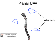
Results
Below is the most exciting result, it is for an airplane with a noisy camera trying to avoid obstacles. Using the verification methods above, we can show that with probability at least $0.99$ that the plane trajectory will not leave the gray region: